Article Text

Abstract
Cardiovascular disease (CVD) is the leading cause of death in women and men. Yet biological and social factors differ between the sexes, while the importance of CVD in women may be underestimated due to the higher age-specific rates in men and the historical bias towards the male model of CVD. Consequently, sex differences in risk factor associations with CVD occur, but these are not always recognised. This article argues that sex disaggregation should be the norm in CVD research, for both humanitarian and clinical reasons. A tutorial on how to design and analyse sex comparisons is provided, including ways of reducing bias and increasing efficiency. This is presented both in the context of analysing individual participant data from a single study and a meta-analysis of sex-specific summary data. Worked examples are provided for both types of research. Fifteen key recommendations are included, which should be considered when undertaking sex comparisons of CVD associations. Paramount among these is the need to estimate sex differences, as ratios of relative risks or differences in risk differences, rather than merely test them for statistical significance. Conversely, when there is no evidence of statistical or clinical significance of a sex difference, the conclusions from the research should not be sex-specific.
- epidemiology
- medical education
- statistics and study design
- meta-analysis
This is an open access article distributed in accordance with the Creative Commons Attribution Non Commercial (CC BY-NC 4.0) license, which permits others to distribute, remix, adapt, build upon this work non-commercially, and license their derivative works on different terms, provided the original work is properly cited, appropriate credit is given, any changes made indicated, and the use is non-commercial. See: http://creativecommons.org/licenses/by-nc/4.0/.
Statistics from Altmetric.com
Rationale for studying sex differences in cardiovascular disease
Historically, cardiovascular disease (CVD) was seen as a disease of men. Nowadays, there is wide recognition that it is also a disease of women, although awareness of coronary heart disease (CHD) as the leading global cause of death in women is lacking both in clinicians and the general public.1 Indeed, CHD and stroke each appear in the top 4 causes of death in both high-income and low-income countries in women as well as in men.1 2
Many authors and activists have done sterling work in raising the profile of female CVD, but often this has involved studies and review articles that report data on women alone. Obviously this is unavoidable if the subject is entirely female—the future risk of CVD in mothers associated with pre-eclampsia during pregnancy, for example—but too often the opportunity of including male controls is missed, leaving open the question of how best to explain the findings from whatever problem the research has investigated. An example comes from a programme of work on women’s reproductive factors and the future risk of CVD in the China Kadoorie Biobank. One potential risk exposure addressed was the number of children to which a woman had given birth.3 Leaving aside the relatively few women who did not have children, risk increased as the number of children increased. Biological mechanisms that suggest such an association include pregnancy-induced alterations in the cardiometabolic system, which previous authors had suggested.4 However, unlike the other female reproductive factors—such as breast feeding—analysed in this programme, the relationship between the number of children and CVD risk could also be explored in the men recruited to the Biobank. Male associations were found to be virtually identical, which suggests that the association is not driven by female biology; this changes the interpretation of the results completely.
Even if the main purpose of the research is not to study female issues in CVD, a strong case can be made for systematic inclusion of sex-specific results in the study’s report. For example, large-scale clinical trials routinely report subgroup analyses, based on demographic and clinical features of the patient population. Even when one sex predominates for the disease under study, sex should be included as one of the subgroup criteria; that is, the association between the randomised intervention and the study outcome(s) should be reported for both women and men. In most cases this should be one of the prespecified subgroup analyses, which provide the strongest evidence that the finding is not due simply to chance, although allowance must be made for the degree of scientific interest in competing patient characteristics, being mindful of the attenuating impact when many subgroup analyses are specified a priori. While acknowledging the possible drawback of irresponsible overinterpretation of underpowered chance findings,5 I consider that sex stratification should be reported even when the chance of finding a sex difference is small. This is so that such results can be used in future meta-analyses.
The case for habitual reporting of results for each sex separately is based on three facts. First, women and men are biologically different, and frequently have different social experiences. Exploring sex differences may, thus, uncover important mechanisms, furthering health and medical research. Second, they each make up approximately 50% of the population, so we can expect sex-specific findings, when distinct, to have widespread relevance—no other factor has such a degree of balance, in general. These are obvious statements, and yet sex-disaggregated results are not (yet) commonplace. For example, when conducting a systematic review of sex-specific associations between smoking and stroke,6 authors found that over 40% of papers, discovered using keywords that included sex-related terms, failed to present associations for women and men separately. This would not matter if there were no sex differences, but the third arm of the case for sex disaggregation is that there are. Women are less likely to demonstrate the ‘classic’ symptoms of CVD,7 which have historically been determined from data on men. Women may thus be misdiagnosed—likely leading to adverse outcomes.8 More generally, failing to consider the sexes independently can cause incorrect inferences to be concluded, with adverse consequences for one or both sexes.9 10 Recognition of these issues has led some research bodies and journals to support, or even mandate, the inclusion of, and reporting of results for, both women and men in research studies.11–14 Although this is far from universal, the contemporary social climate, at least in the Western world, suggests that reporting of results by sex may well become routine in future medical research.
Practical considerations often mean that one cannot balance the sex representation in a study. In an ideal world the same number of women and men would be recruited into all cardiovascular trials, with sex being one of the factors on which randomisation is stratified. But, just as in the case of prespecified subgroups, other factors may trump sex for prognostic value, given that few factors can realistically be allowed for in randomisation. The result may well be a sex imbalance. In epidemiological studies, the sex ratio will typically be dictated by the study population at large, or that of the subpopulation of cases of the index disease. Analyses of sex differences using unequal numbers of women and men are less efficient than otherwise, but this is certainly not a terminal problem.
Tutorial for analysing and reporting sex differences in cardiovascular associations
Sex and gender
I am taking ‘sex’ to be the dichotomy between women and men. For behavioural risk factors, ‘sex’ would usually be replaced by ‘gender’, but I make no such distinction in this exposition because the methodologies would be the same. Should sex or gender be considered non-binary (as they undoubtedly are), things get more complicated, although once one group is considered to be the reference group generalisations can be made. Similarly, I am restricting myself to examining sex-specific associations between a binary risk factor (eg, obese vs not) and the risk of CVD. The same methods will often apply if the risk factor is considered in a linear continuous way (eg, per 5 kg/m2 body mass index), on the log scale. Should the risk factor be categorical, or at least considered in this fashion (eg, underweight/normal weight/overweight/obese), one group should be considered as the reference (eg, normal weight) and the methods presented here can, again, be generalised by analysing a set of comparisons with the common reference.
Comparison of risk
When studying associations between a risk factor and CVD, the most basic summary statistics are the risks of CVD in the risk factor-positive (exposed) and risk factor-negative (unexposed) subgroups. If the study is prospective with no (or, at least, insignificant) loss to follow-up (censoring), then both risks are relative frequencies (see table 1 for examples). When censoring occurs (due to a death from a non-CVD cause or due to emigration), it is best to allow for it by using the rate, for example per thousand person-years of observation, to estimate the risk.
Fundamental metrics of risk
Risks can be compared on the relative or absolute scale. Comparisons are typically made, respectively, using the relative risk (RR) and risk difference (RD)—see table 1. When one considers that the risk is itself a relative parameter (eg, the number of myocardial infarction (MI) events divided by the number at risk), use of the RR has the advantage of maintaining consistency. RRs and, most tellingly, their variances are also easier than RDs to obtain from standard software, and consequently are much more common in medical literature. Finally, they travel well, in the sense that an RR for a given risk factor—disease association in one study population is likely to be a reasonable estimate of the same association in another population. However, experience shows that typical RRs in CVD research vary with age15 (eg, see figure 1), so this advantage may be limited to populations with similar age structures. On the other hand, RDs tend to be heterogeneous. They are more useful for making clinical decisions in a specific population, particularly because they can be used to determine the expected number that will experience the outcome studied over a fixed time period. Several eminent epidemiologists have championed their use.16
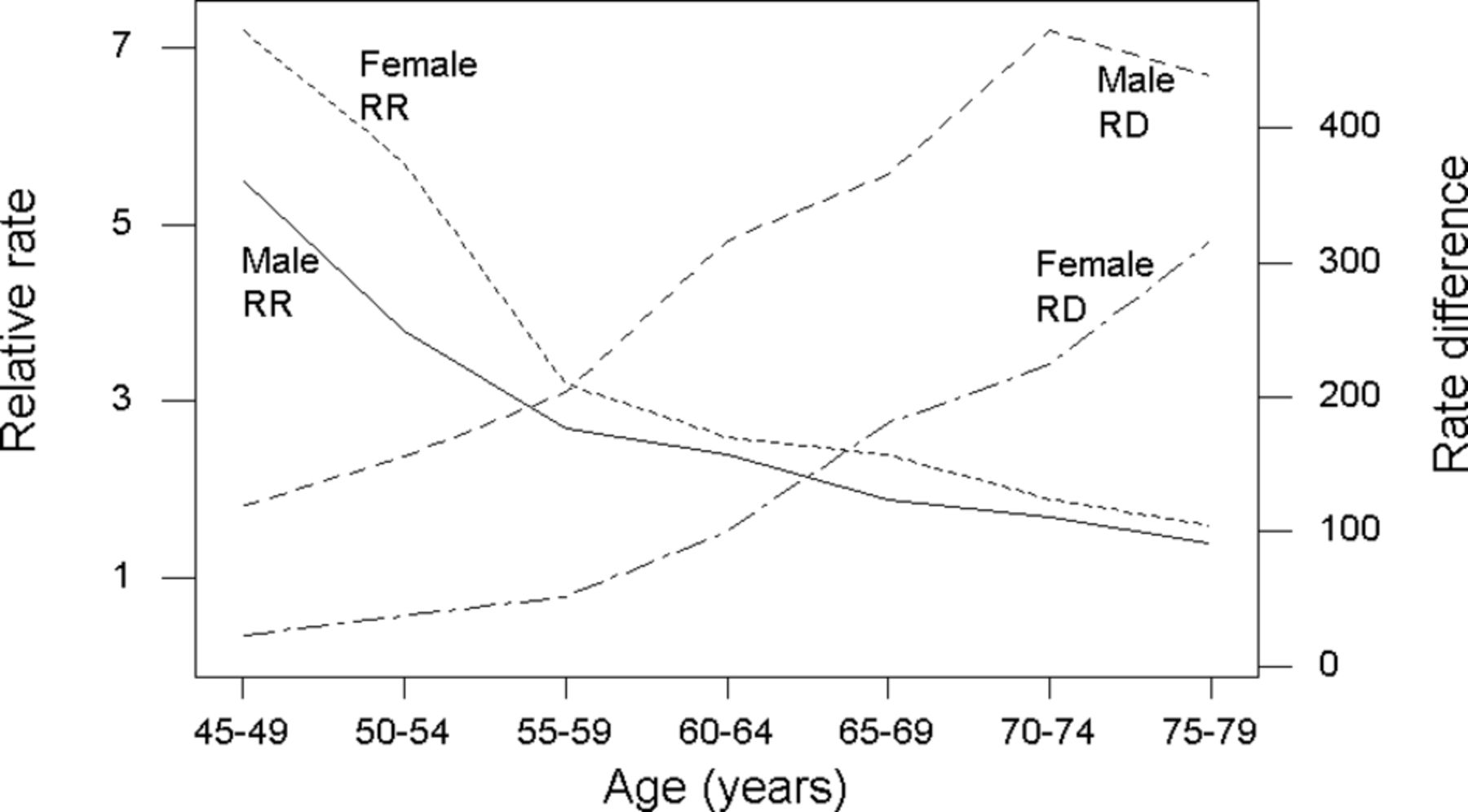
Relative rate (RR) and rate difference (RD) (per 100 000 per year) for coronary heart disease by age group (45–79 years old) and sex, comparing smokers to never-smokers (American Cancer Prevention Study II, National Cancer Institute, 1997). Figure reproduced from Woodward (Epidemiology: Study Design and Data Analysis, Third Edition17 and Second Edition, 2005).
It may well be sensible to analyse the same set of data on both the relative and absolute scales to enable a full set of inferences and interpretations. For instance, in figure 1, when moving from RRs to RDs, not only do the sex-specific patterns in trends by age interchange position (women doing worse for RRs but better for RDs, at all ages) but also so does the direction of trend (RR decreases with age; RD increases).17
Here, I am concerned with comparing an association, say between obesity and CVD, between the sexes. This leads to consideration of the ratio of RRs—the RRR—and the difference in RDs—the DRD, as defined in table 1. Since women typically suffer CVD 5–10 years later than men, in all but the most elementary analyses, adjustment by age is essential to obtain meaningful inferences regarding sex differences. We might also like to adjust for other CVD risk factors thought to be confounders. Hence statistical models will be used.
Analysing sex differences using the individual participant data from a single study
Sex comparisons on the relative scale
We can easily analyse the sex-specific portions of individual participant data (IPD) separately to get female and male RRs, which is what many authors do. Having done that, they will often fit the interaction model, for example the model with sex (female/male), obesity (yes/no) and their interaction, to test whether the sex difference is significant. Note that this interaction model should also include all main effects and sex interactions for each confounding variable included in the sex-specific models, otherwise the adjustments made in the interaction model will not vary by sex, as they do in the sex-specific models. However, p values have limited utility, and it is more practically useful to estimate the RRR (and 95% CI) for the sex difference (eg, in the effect of obesity on CVD), stating clearly whether women are compared with men, or vice versa (maintaining consistency, should several similar analyses be conducted in the same study). While the estimated RRR arises from a simple division, deriving its 95% CI from the sex-specific 95% CIs (and estimates) is time-consuming (as described later in the context of a meta-analysis) and inaccurate. Instead, the 95% CI can be found from the computer output when fitting the interaction model; it will usually be given alongside the p value. Note that some computer packages will give results on the logarithmic scale, thus producing ln(RR)s and the ln(RRR), where ln denotes log to the exponential base. Exponential transformations are then required to obtain final results.
An alternative approach is to use the interaction model to obtain the RRs as well as the RRR. This works because the interaction model will directly produce the RR for whichever sex is taken as the reference group, as well as the RRR comparing the other sex with the reference sex. So, if men are taken as the reference group, we would get the male RR and the female to male RRR (as well as their 95% CIs) straight from the computer output. To get the female RR from the same computer output is quite easy, but getting its 95% CI is less straightforward since covariances must be dealt with. A simple trick, to avoid this issue, is to interchange the codes given to the sex variable (often 0 and 1), thus making the other sex now the reference group, and run the interaction model again. Continuing the example, this second run would produce the female RR and the male to female RRR (and 95% CI). We are unlikely to want the latter, since it is simply the reciprocal of the female to male RRR (the same is true of the confidence limits, once they are interchanged).
I prefer to use the interaction model to obtain the RRs and RRR because it requires fewer models to be fit. Also, using the interaction model alone ensures that results for the ratio of sex-specific RRs and the RRR must be completely concordant.
Worked example
Consider the problem of estimating the RRs by sex and the female to male RRR when relating diabetes to the risk of MI, adjusting for age, systolic blood pressure and smoking status. Using data from the UK Biobank, I selected all people without CVD at baseline, except those (relatively few) with missing values, and fitted Cox proportional hazards regression models in the Stata package (V.15); the code and results appear in online supplementary appendix 1. Using sex-specific models, the RRs for MI (diabetes vs not) were 2.97 (95% CI 2.53 to 3.48) for women and 1.66 (95% CI 1.49 to 1.84) for men over a 7-year follow-up period. The female to male RRR was thus 2.97/1.66=1.79. The interaction model (with men as the reference group) gave the RR for men as 1.66 (95% CI 1.49 to 1.84) and the female to male RRR as 1.79 (95% CI 1.48 to 2.17). Swapping to use of women as the reference group gave the RR for women as 2.97 (95% CI 2.53 to 3.48). So both methods give the same results, but use of the interaction model alone (here fitted twice) saved one model fitting exercise compared with the sex-specific approach (which needs one run of the interaction model to get the 95% CI for the RRR). In Stata, and some other software, it is possible to get all the three statistics of interest, with CIs, directly by fitting the interaction model just once (see online supplementary appendix 1). Whatever the approach, we conclude that diabetes, after adjustment, increases the risk of MI in both sexes, but the relative increase is about 80% bigger in women. Note that because Cox models were used, strictly speaking, the results here are HRs and their quotient (see notes to table 1).
Supplemental material
Sex comparisons on the absolute scale
On the absolute scale, when survival data are analysed, it is usual to use rates per person-year to express risk. Sex-specific RDs and the DRD derive from Poisson regression models, taking the logarithm of the follow-up time (per individual), suitably scaled (so that results, for example, per 10 000 person-years, are produced) as an offset.17 Fitting a Poisson model with sex as the only input variable gives the sex-specific rates in the study population—although these are easy to compute by hand, Poisson regression also gives the accompanying CIs.
Worked example
Using the same UK Biobank data as before, online supplementary appendix 2 shows the results from fitting Poisson regression models in Stata. The rates of MI were found to be 7.90 and 24.64 per 10 000 person-years for women and men, respectively. This puts the risk of MI in perspective—for every thousand women followed up for 10 years, we would expect about 8 to get MI, and for every thousand men we would expect about 25. Fitting models for sex differences relating diabetes to MI produced estimates of rates (and their CIs; approximately evaluated using the delta method in Stata). Table 2 shows both the unadjusted and adjusted rates, using the same adjustments as when RRs were estimated previously. This shows that women, and those without diabetes, have the lower rates, and adjustment only has any appreciable effect for men with diabetes—the group at most risk. Simple subtractions show that diabetes is associated with roughly one extra MI case per 10 000 person-years of observation in women compared with men. Despite the much higher RR in women found earlier, the difference in additional expected MI cases associated with diabetes is negligible in this study population (without previous CVD and otherwise relatively healthy), partially because the overall risk of MI is low. Should the RRR stay the same in high-risk subpopulations, we would expect much higher numbers of excess female cases of MI.
Rates of myocardial infarction, per 10 000 person-years, in a subsample of the UK Biobank without cardiovascular disease at baseline
See Millett et al 15 for a comprehensive study of sex differences in risk factors for MI in the UK Biobank using the same methods described here.
Incidentally, the Poisson model can also be used to estimate the RRs and RRR, as an alternative to the Cox model. Comparison of fitted parameter estimates for the adjusted models in online supplementary appendices 1 and 2 shows very similar estimates and 95% CIs. A simple way of seeing the linkage between the two approaches is to compute the adjusted RRs and the RRR from the results in the right-hand side of table 2, which gives the RRs as 2.97 (women) and 1.66 (men), with the RRR of 1.79, just as was found from the Cox model.
Analysing sex differences using summary data from multiple studies
A number of different studies may have published sex-disaggregated results linking the risk factor of our interest to the outcome of our interest. It would then make sense to summarise their findings using meta-analysis, starting from a systematic review of the literature (possibly including unpublished sources and certainly including citation tracing from original sources). Suppose that every study has an estimate of the RR (per sex), and these are what we wish to summarise, through pooling. As a motivating example, I will take the study of Peters et al.18 The authors compiled data from 19 studies which provided sex-specific RRs for CHD, comparing those with diabetes to those not; two of these studies provided RRs in two separate subgroups of their total study population, giving 21 RRs to pool in all, for each sex (table 3).
Multiple-adjusted coronary heart disease relative risks (and 95% CIs) for women and men, comparing those with, to those without, diabetes, by study
Since our goal is to compare the sexes, it is best to only include studies with results for both women and men. This is because differences in the make-up of study populations, definitions of the exposure and outcome, and the methods of analysis might introduce bias error if single-sex studies are included in the pooling process. For instance, published studies must be expected to include a range of adjustment sets; the data in table 3 come from studies which adjusted for confounding factors in many ways, with between 5 and 10 factors included (see figure 2). By only including studies with results from both sexes, we ensure that between-study variations (known or unknown) will be the same for women and men. Another general exclusion, which I would advise, is studies that do not adjust at least for age. Often other classical risk factors for CHD will also be adjusted for in published studies, but being too prescriptive in what must be included or excluded can lead to few studies being selected for pooling. If we have access to IPD, we can decide on our own adjustments. Indeed, four of the RR pairs in table 3 came from IPD analyses, adjusting diabetes for age, systolic blood pressure, smoking, body mass index and serum total cholesterol in each case.
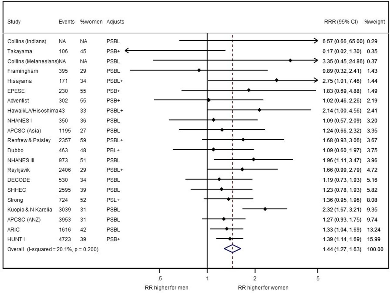
Women to men ratios of coronary heart disease relative risks (RRRs), comparing those with, to those without, diabetes, by study and pooled overall. Data are from table 3. Random effects inverse variance weighting was used to pool the study-specific data. Horizontal lines show 95% CIs, as does the width of the summary diamond. ‘Events’ are of coronary heart disease during follow-up (some studies only recorded fatal coronary events), and ‘%women’ gives the percentage of these events that were female. ‘NA’ denotes ‘not available’. ‘Adjusts’ gives the summary details of the adjustments made, per study: P denotes blood pressure (which is most often systolic, but sometimes is hypertension or antihypertensive use; in one study adjustments were made for both diastolic and systolic blood pressure); S denotes smoking; B denotes body mass index; L denotes lipids (which always included total cholesterol, but sometimes also other lipids); + denotes other coronary risk factors. The p value is for a test of no heterogeneity.17 RR, relative risk; RRR, ratio of RR.
Study pooling
To obtain an overall picture of the sex-specific association between the exposure and the disease (diabetes and CHD, in the example), meta-analysis can be used to estimate the pooled RR, across all studies, for women and for men. There are many ways that such pooling can be achieved.17 For example, we could take a simple mean of the separate study estimates, but this would not account for any differences in quality (relative lack of bias) or quantity (precision; relative lack of sampling error) between the constituent studies. So a weighted mean is preferred. In practice, most meta-analyses weight by precision and leave bias to be assessed more informally using standard criteria, such as the Newcastle-Ottawa Scale,19 independent of the pooling process.
The most popular weighting scheme is inverse variance (IV) weighting—as the name suggests, each study is weighted by the reciprocal of its variance. This makes sense because the less precise the study, the larger will be its variance (and the wider will be the CI around the point estimate of the RR). Subsequently all weights are transformed to sum to 100%, for easy interpretation, by dividing each individual weight by the sum of all the weights and multiplying by 100. An advantage of IV weighting is that it produces the narrowest possible CI for the pooled RR. A drawback, shared by other popular weighting schemes, is that it can only be applied to studies for which some measure of the variability associated with the study’s estimate is available. Generally published studies report the SE of the estimate (ie, the square root of the variance) or a 95% CI. To pool results we need the same metric for all studies; suppose we decide to use the SEs. We may then need to derive SEs from published 95% CIs in some cases. This requires, first, taking logarithms of the estimate and the 95% confidence limits. This is necessary because, although the RR itself does not have the classic normal form, its logarithm, ln(RR), is approximately normally distributed. That being so, we know that the 95% CI must have the form17:

where E is the point estimate, ln(RR), and SE is the SE of the ln(RR). This means that

where L and H are the lower and higher 95% confidence limits, respectively, of the ln(RR). In practice, these two equations will give different answers for the SE, if only due to rounding errors in L and H. If they are very different we should check our arithmetic and refer back to the source document for confirmation (numerical errors in published works have been known to occur). The two results should be averaged to find the ‘best’ estimate of the SE (see table 4, example 1).
Worked examples using the first study in table 3 (the Adventist study)
Once we have estimates, and their variability, these can easily be pooled. The computations are not complex for IV weighting17 and could be applied in Excel. However, most researchers will want to use software, not least to be able to produce graphical displays. A range of specialist software exists,20 but I prefer to use the user-supplied Stata procedure metan. This procedure allows the user to enter either the estimate and its SE or the estimate and its 95% CI (or a CI of a different degree) from each study to commence pooling and assumes that the estimate follows a (near) normal distribution, at least for the type of data addressed here. As already discussed, the RR does not follow this form, so when meta-analysing RRs we should instead pool ln(RR)s. The eform option should be included in the metan command as this back-transforms the natural logs of the pooled RR, and its confidence limits, to the natural scale, in the presentation of results.
Fixed effect and random effects
This account of meta-analysis, so far, has implicitly assumed the fixed effect approach. This assumes that there is a universal true RR for women (and for men) which relates to all studies, wherever, or whenever, they were conducted. The variation between estimates is attributed solely to study-specific sampling error—that is, the difference between the sample and its source population. Many, but not all, authors prefer the random effects approach which allows the true RR to vary by study and interprets the pooled estimate as the average of all the different ‘truths’.17 Random effects allows for greater uncertainty and thus will produce 95% CIs for the pooled RR that are at least as big as for the corresponding fixed effect analysis. To the practitioner, the advantage of random effects is that it will give the same result as fixed effect if there is no between-study heterogeneity, so in this sense it is the safe option. It operates like IV weighting, as it has been described above, but where an additional component is added to the variance for each study to account for between-study heterogeneity. That is, fixed effect weights a study by 1/V, where V is that study’s variance, but random effects weights by 1/(U+V), where U is the between-study variance (computed from a complex formula17 21; omitted here). As a consequence, the random effects approach gives less weight to the biggest (in terms of outcome events) cohort studies than does the fixed effect.
Putting the data from table 3 into Stata, using the metan procedure to pool the RRs for each sex, produced the results in table 5. As can be seen, similar results pertained whether fixed effect or random effects was used. It is also very clear that the RR for women is larger than that for men, suggesting that diabetes is a stronger risk factor for CHD in women than in men. An estimate of the percentage of variability attributable to between-study heterogeneity, called the i-squared statistic,17 21 has been included in table 5. Some researchers use this to decide whether to apply fixed effect or random effects, often using 25% as a threshold above which between-study heterogeneity is thought to be too great for the fixed effect assumption to be viable. Others, including me, feel that the choice should be made a priori. As in all cases, methods decided on before the data are analysed will be more defensible.
Inverse variance weighted pooled relative risks and ratios of relative risks (with 95% CIs) for the association between diabetes and coronary heart disease
The ratio of relative risks
So far, no mention has been made of sex comparisons, which can be made through the women to men RRR. Given the female and male RRs, the RRR is straightforward to derive per study, but to pool the RRRs using IV weighting requires knowledge of the variance (or similar) of the RRR in each study. These are simple to estimate once we transform to the log scale, which converts the problem from dealing with ratios to one dealing with differences. The variance of the difference in ln(RR)s between women and men is the sum of the variances of the female and male ln(RR)s, and the SE of the difference is its square root. Since this difference can reasonably be assumed to follow a normal distribution, we can compute the 95% CI for the ln(RRR), if required, using the formulae given above, and use metan to pool the ln(RRR)s across studies. Table 4 (example 2) has the calculation for the first study in table 3, and online supplementary appendix 3 is a copy of the Excel file used to make computations for all 21 studies (or part studies).
Pooling of RRRs across studies then proceeds in the same way as for the RRs, that is, pooling on the log scale and back-transforming the pooled estimate and 95% confidence limits. Figure 2 is a forest plot17 21 of the individual study and random effects IV weighted pooled results. To produce this plot I used metan in Stata, having input the 21 ln(RRR)s, and their SEs, from online supplementary appendix 3, augmented by some additional study characteristics for enhanced interpretation, as presented in online supplementary appendix 4. The Stata code and results appear in online supplementary appendix 5, while table 5 includes summary results from both fixed effect and random effects analyses. I did minor artistic editing of the Stata graph in PowerPoint.
Forest plots are extremely useful for presenting the results of a meta-analysis, as well as in other settings; for example, Millett et al 15 used them to compare sex differences in MI across a range of risk factors. Rather than simply order the lines in the plot alphabetically (as would be common in a list of studies), more information is gleamed if they are ordered by study weight, as in figure 2, or according to some important feature of the data, such as year of study publication. However, when female and male results are shown alongside each other, a common ordering aids interpretation. Peters et al 18 included a forest plot ordered by the size of the estimated RRR, which is also informative and makes for, arguably, the most visually attractive presentation. These authors18 also included a box around each study’s estimate, with boxes drawn in proportion to the precision of the study (ie, the IV). This offers an additional visual idea of the relative weight contributed by each study to the pooled estimate.
From figure 2, we conclude that, although diabetes increases the risk of CHD in both sexes, women have a 44% higher RR for CHD related to diabetes than men. We are 95% confident that the range from 27% to 63% contains the true excess RR. Since this interval omits 0% by a considerable degree, there is statistical evidence of a real sex difference.
Notice that when the female RR given in table 5 is divided by the corresponding male RR, the result is not quite the same as the RRR produced by pooling. This is not unexpected, but is rarely an issue since the two tend to be very similar, as here.
Other considerations in report writing
In manuscripts, a flow chart describing the systematic review that identified the data used in the meta-analysis is essential. I would also recommend showing female-specific and male-specific RRs, as well as RRRs, in forest plots. This is both because the sex-specific results are themselves of interest and because it makes the RRRs easier to understand. Comparing age-adjusted and multiple-adjusted results may provide another insightful contrast.
As with all meta-analyses, investigation of the causes of heterogeneity is essential through subgroup analyses and meta-regression, with accompanying bubble plots.17 22–24 Typical factors to investigate as causes of heterogeneity in the RRRs are age, year(s) of study, length of follow-up, risks (overall average or their female to male difference) and the prevalence of the index risk factor (again, overall or as a sex contrast), but what is possible is driven by the published data and thus hard to decide completely a priori. It is also useful to identify any influential studies and investigate possible publication bias, taking remedial action where appropriate.17 22
Other metrics of sex difference
In cases where ORs, HRs or relative rates are to be pooled, the same methods as above can be used to obtain the sex-specific results and the sex comparison (eg, through the ratio of ORs). Indeed, meta-analyses often pool published results claimed to be RRs from studies which have used different metrics to measure relative associations. In most cases this is very reasonable, but care is required if ORs are mixed with other metrics, because the OR overestimates the RR. The general rule is that the OR is an acceptable proxy for the RR if the outcome analysed is rare, which is the case for CVD in most general populations. However, this is usually not the case when comparing the prevalence of anti-CVD medication use between the sexes in secondary prevention. Better, then, to show pooled results separately for each metric used.25
When analyses and inferences on the absolute scale are envisaged, the RD would be the measure of association in each sex, and the sex effect would be estimated by the DRD. Unfortunately pooling is rarely justified in this case because risk tends to be extremely variable between study populations and over time. For instance, while one might reasonably hypothesise that the RRs, comparing those with and without diabetes, for CHD are similar across the world, it is much more of a stretch to think that the rate of CHD per 10 000 person-years in those with (or without) diabetes is very similar in relatively poor and relatively rich countries, or the same 50 years ago as now in the same country. In the vast majority of cases there is too much heterogeneity to make pooled estimates of risk, or RD, meaningful (no average could have a useful meaning). Another problem is that most published studies do not provide the necessary statistics for meta-analyses; they may not even state the sex-specific risks with and without the risk factor of interest, and associated variability. Sometimes the only way of bringing in issues of absolute effects is to follow a meta-analysis on the RRRs with meta-regression of the RRRs on the CVD risks, or their differences by sex, for those studies which provide them, to decide whether the pooled RRR can reasonably be assumed to represent most scenarios.
Conclusions
Sex disaggregation of research findings is strongly encouraged. Methods employed to investigate, and compare, sex-specific associations are generally straightforward, but interpretation can require some careful thinking. Unveiling a sex difference naturally leads to investigation of its cause, which is a natural extension of the subject matter described in this manuscript. For example, the excess proportionate risk of heart disease associated with diabetes in women, compared with men, found here in two distinct research databases, leads to further research into the cause.26
A summary of my recommendations appears in table 6. This may serve as a useful checklist when undertaking sex differences research in CVD. Stata and Excel files used in my analyses are given in the online supplementary material.
Recommendations
Acknowledgments
I would like to acknowledge my adaption of the computer code devised by the late Dr Elizabeth Millett when preparing her work on the UK Biobank (15). This research has used the UK Biobank Resource (application No 2495). Permission to use the UK Biobank Resource was approved by the access subcommittee of the UK Biobank Board.
References
Footnotes
Contributors MW wrote the entire paper.
Funding MW is supported by a National Health and Medical Research Council Fellowship (APP108026) and Program Grant (APP1149987). The funding sources had no role in the design or conduct of the study; collection, management, analysis and interpretation of the data; or preparation, review or approval of the manuscript.
Competing interests MW does consultancy for Amgen and Kyowa Hakko Kirin outside the submitted work.
Ethics approval UK Biobank has obtained research tissue bank approval from its governing research ethics committee, as recommended by the National Research Ethics Service. No separate ethical approval was required. The study was conducted in accordance with the principles of the Declaration of Helsinki.
Provenance and peer review Not commissioned; externally peer reviewed.
Data sharing statement Researchers can apply to use the UK Biobank resource and access the data used. No additional data are available.
Patient consent for publication Not required.