Prognosis and prognostic research: Developing a prognostic model
BMJ 2009; 338 doi: https://doi.org/10.1136/bmj.b604 (Published 31 March 2009) Cite this as: BMJ 2009;338:b604
- Patrick Royston, professor of statistics1,
- Karel G M Moons, professor of clinical epidemiology2,
- Douglas G Altman, professor of statistics in medicine3,
- Yvonne Vergouwe, assistant professor of clinical epidemiology2
- 1MRC Clinical Trials Unit, London NW1 2DA
- 2Julius Centre for Health Sciences and Primary Care, University Medical Centre Utrecht, Utrecht, Netherlands
- 3Centre for Statistics in Medicine, University of Oxford, Oxford OX2 6UD
- Correspondence to: P Royston pr{at}ctu.mrc.ac.uk
- Accepted 6 October 2008
The first article in this series reviewed why prognosis is important and how it is practised in different medical settings.1 We also highlighted the difference between multivariable models used in aetiological research and those used in prognostic research and outlined the design characteristics for studies developing a prognostic model. In this article we focus on developing a multivariable prognostic model. We illustrate the statistical issues using a logistic regression model to predict the risk of a specific event. The principles largely apply to all multivariable regression methods, including models for continuous outcomes and for time to event outcomes.
Summary points
Models with multiple variables can be developed to give accurate and discriminating predictions
In clinical practice simpler models are more practicable
There is no consensus on the ideal method for developing a model
Methods to develop simple, interpretable models are described and compared
The goal is to construct an accurate and discriminating prediction model from multiple variables. Models may be a complicated function of the predictors, as in weather forecasting, but in clinical applications considerations of practicality and face validity usually suggest a simple, interpretable model (as in box 1).
Box 1 Example of a prognostic model
Risk score from a logistic regression model to predict the risk of postoperative nausea or vomiting (PONV) within the first 24 hours after surgery2:
Risk score= −2.28+(1.27×female sex)+(0.65×history of PONV or motion sickness)+(0.72×non-smoking)+(0.78×postoperative opioid use)
where all variables are coded 0 for no or 1 for yes.
The value −2.28 is called the intercept and the other numbers are the estimated regression coefficients for the predictors, which indicate their mutually adjusted relative contribution to the outcome risk. The regression coefficients are log(odds ratios) for a change of 1 unit in the corresponding predictor.
The predicted risk (or probability) of PONV=1/(1+e−risk score).
Surprisingly, there is no widely agreed approach to building a multivariable prognostic model from a set of candidate predictors. Katz gave a readable introduction to multivariable models,3 and technical details are also widely available.4 5 6 We concentrate here on a few fairly standard modelling approaches and also consider how to handle continuous predictors, such as age.
Preliminaries
We assume here that the available data are sufficiently accurate for prognosis and adequately represent the population of interest. Before starting to develop a multivariable prediction model, numerous decisions must be made that affect the model and therefore the conclusions of the research. These include:
Selecting clinically relevant candidate predictors for possible inclusion in the model
Evaluating the quality of the data and judging what to do about missing values
Data handling decisions
Choosing a strategy for selecting the important variables in the final model
Deciding how to model continuous variables
Selecting measure(s) of model performance5 or predictive accuracy.
Other considerations include assessing the robustness of the model to influential observations and outliers, studying possible interaction between predictors, deciding whether and how to adjust the final model for over-fitting (so called shrinkage),5 and exploring the stability (reproducibility) of a model.7
Selecting candidate predictors
Studies often measure more predictors than can sensibly be used in a model, and pruning is required. Predictors already reported as prognostic would normally be candidates. Predictors that are highly correlated with others contribute little independent information and may be excluded beforehand.5 However, predictors that are not significant in univariable analysis should not be excluded as candidates.8 9 10
Evaluating data quality
There are no secure rules for evaluating the quality of data. Judgment is required. In principle, data used for developing a prognostic model should be fit for purpose. Measurements of candidate predictors and outcomes should be comparable across clinicians or study centres. Predictors known to have considerable measurement error may be unsuitable because this dilutes their prognostic information.
Modern statistical techniques (such as multiple imputation) can handle data sets with missing values.11 12 However, all approaches make critical but essentially untestable assumptions about how the data went missing. The likely influence on the results increases with the amount of data that are missing. Missing data are seldom completely random. They are usually related, directly or indirectly, to other subject or disease characteristics, including the outcome under study. Thus exclusion of all individuals with a missing value leads not only to loss of statistical power but often to incorrect estimates of the predictive power of the model and specific predictors.11 A complete case analysis may be sensible when few observations (say <5%) are missing.5 If a candidate predictor has a lot of missing data it may be excluded because the problem is likely to recur.
Data handling decisions
Often, new variables need to be created (for example, diastolic and systolic blood pressure may be combined to give mean arterial pressure). For ordered categorical variables, such as stage of disease, collapsing of categories or a judicious choice of coding may be required. We advise against turning continuous predictors into dichotomies.13 Keeping variables continuous is preferable since much more predictive information is retained.14 15
Selecting variables
No consensus exists on the best method for selecting variables. There are two main strategies, each with variants.
In the full model approach all the candidate variables are included in the model. This model is claimed to avoid overfitting and selection bias and provide correct standard errors and P values.5 However, as many important preliminary choices must be made and it is often impractical to include all candidates, the full model is not always easy to define.
The backward elimination approach starts with all the candidate variables. A nominal significance level, often 5%, is chosen in advance. A sequence of hypothesis tests is applied to determine whether a given variable should be removed from the model. Backward elimination is preferable to forward selection (whereby the model is built up from the best candidate predictor).16 The choice of significance level has a major effect on the number of variables selected. A 1% level almost always results in a model with fewer variables than a 5% level. Significance levels of 10% or 15% can result in inclusion of some unimportant variables, as can the full model approach. (A variant is the Akaike information criterion,17 a measure of model fit that includes a penalty against large models and hence attempts to reduce overfitting. For a single predictor, the criterion equates to selection at 15.7% significance.17)
Selection of predictors by significance testing, particularly at conventional significance levels, is known to produce selection bias and optimism as a result of overfitting, meaning that the model is (too) closely adapted to the data.5 9 17 Selection bias means that a regression coefficient is overestimated, because the corresponding predictor is more likely to be significant if its estimated effect is larger (perhaps by chance) rather than smaller. Overfitting leads to worse prediction in independent data; it is more likely to occur in small data sets or with weakly predictive variables. Note, however, that selected predictor variables with very small P values (say, <0.001) are much less prone to selection bias and overfitting than weak predictors with P values near the nominal significance level. Commonly, prognostic data sets include a few strong predictors and several weaker ones.
Modelling continuous predictors
Handling continuous predictors in multivariable models is important. It is unwise to assume linearity as it can lead to misinterpretation of the influence of a predictor and to inaccurate predictions in new patients.14 See box 2 for further comments on how to handle continuous predictors in prognostic modelling.
Box 2 Modelling continuous predictors
Simple predictor transformations intended to detect and model non-linearity can be systematically identified using, for example, fractional polynomials, a generalisation of conventional polynomials (linear, quadratic, etc).6 27 Power transformations of a predictor beyond squares and cubes, including reciprocals, logarithms, and square roots are allowed. These transformations contain a single term, but to enhance flexibility can be extended to two term models (eg, terms in log x and x2). Fractional polynomial functions can successfully model non-linear relationships found in prognostic studies. The multivariable fractional polynomial procedure is an extension to multivariable models including at least one continuous predictor,4 27 and combines backward elimination of weaker predictors with transformation of continuous predictors.
Restricted cubic splines are an alternative approach to modelling continuous predictors.5 Their main advantage is their flexibility for representing a wide range of perhaps complex curve shapes. Drawbacks are the frequent occurrence of wiggles in fitted curves that may be unreal and open to misinterpretation28 29 and the absence of a simple description of the fitted curve.
Assessing performance
The performance of a logistic regression model may be assessed in terms of calibration and discrimination. Calibration can be investigated by plotting the observed proportions of events against the predicted risks for groups defined by ranges of individual predicted risks; a common approach is to use 10 risk groups of equal size. Ideally, if the observed proportions of events and predicted probabilities agree over the whole range of probabilities, the plot shows a 45° line (that is, the slope is 1). This plot can be accompanied by the Hosmer-Lemeshow test,19 although the test has limited power to assess poor calibration. The overall observed and predicted event probabilities are by definition equal for the sample used to develop the model. This is not guaranteed when the model’s performance is evaluated on a different sample in a validation study. As we will discuss in the next article,18 it is more difficult to get a model to perform well in an independent sample than in the development sample.
Various statistics can summarise discrimination between individuals with and without the outcome event. The area under the receiver operating curve,10 20 or the equivalent c (concordance) index, is the chance that given two patients, one who will develop an event and the other who will not, the model will assign a higher probability of an event to the former. The c index for a prognostic model is typically between about 0.6 and 0.85 (higher values are seen in diagnostic settings21). Another measure is R2, which for logistic regression assesses the explained variation in risk and is the square of the correlation between the observed outcome (0 or 1) and the predicted risk.22
Example of prognostic model for survival with kidney cancer
Between 1992 and 1997, 350 patients with metastatic renal carcinoma entered a randomised trial comparing interferon alfa with medroxyprogesterone acetate at 31 centres in the UK.23 Here we develop a prognostic model for the (binary) outcome of death in the first year versus survived 12 months or more. Of 347 patients with follow-up information, 218 (63%) died in the first year.
We took the following preliminary decisions before building the model:
We chose 14 candidate predictors, including treatment, that had been reported to be prognostic
Four predictors with more than 10% missing data were eliminated. Table 1⇓ shows the 10 remaining candidate predictors (11 variables).
WHO performance status (0, 1, 2) was modelled as a single entity with two dummy variables
For illustration, we selected the significant predictors in the model using backward elimination with the Akaike information criterion17 and using 0.05 as the significance level. We compared the results with the full model (all 10 predictors)
Because of its skew distribution, time to metastasis was transformed to approximate normality by adding 1 day and taking logarithms. All other continuous predictors were initially modelled as linear
For each model, we calculated the c index and receiver operating curves and assessed calibration using the Hosmer-Lemeshow test.
Selected predictors of 12 month survival for patients with kidney cancer. Estimated mutually adjusted regression coefficient (standard error) for three multivariable models obtained using different strategies to select variables (see text)
Table 1⇑ shows the full model and the two reduced models selected by backward elimination using the Akaike information criterion and 5% significance. Positive regression coefficients indicate an increased risk of death over 12 months. None of the three models failed the Hosmer-Lemeshow goodness of fit test (all P>0.4).
Two important points emerge. Firstly, larger significance levels gave models with more predictors. Secondly, reducing the size of the model by reducing the significance level hardly affected the c index. Figure 1⇓ shows the similar receiver operating curves for the three models. We note, however, that the c index has been criticised for its inability to detect meaningful differences.24 As often happens, a few predictors were strongly influential and the remainder were relatively weak. Removing the weaker predictors had little effect on the c index.

Fig 1 Receiver operating characteristic (ROC) curves for three multivariable models of survival with kidney cancer.
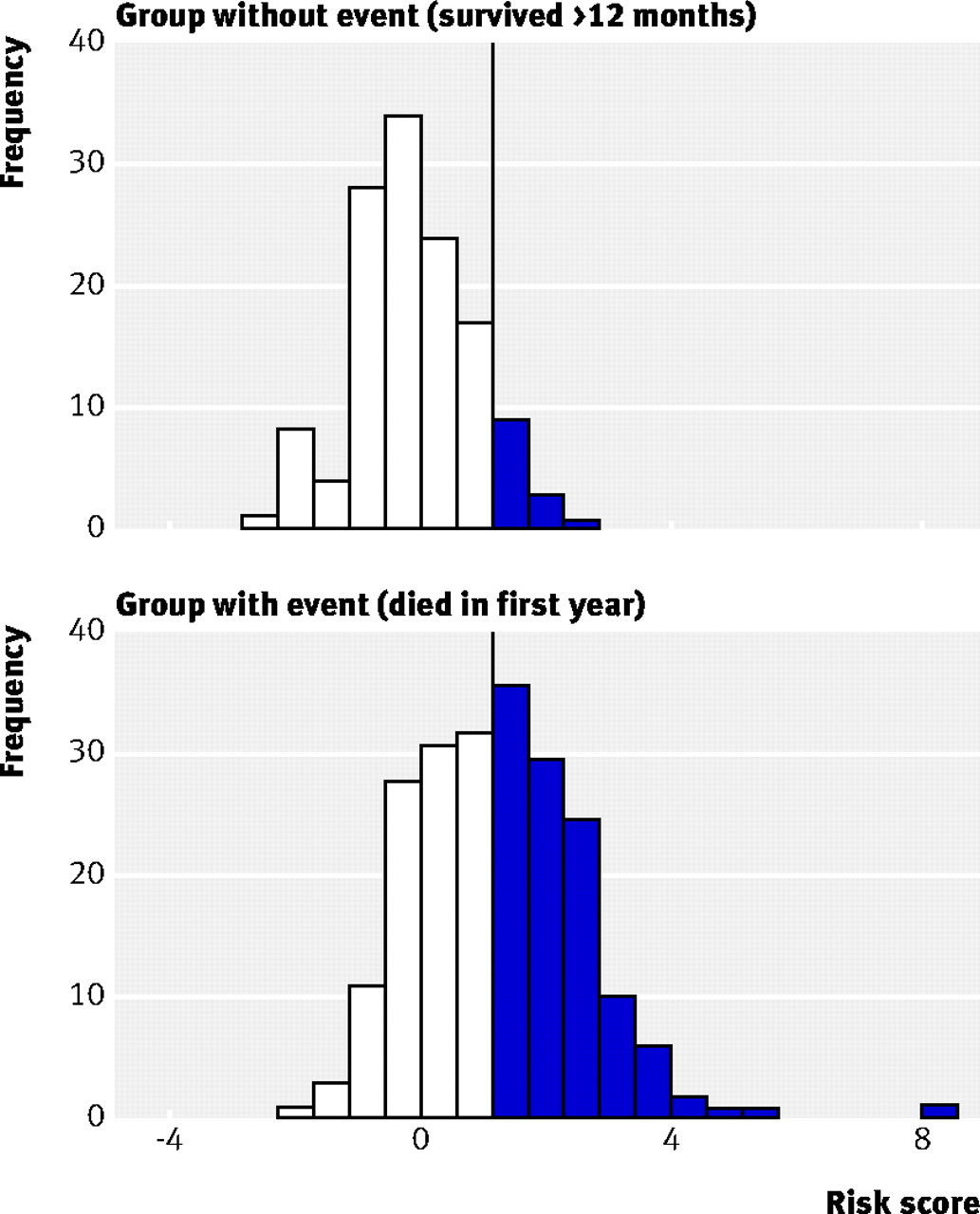
An important goal of a prognostic model is to classify patients into risk groups. As an example, we can use as a cut-off value a risk score of 1.4 with the full model (vertical line, fig 2⇓) which corresponds to a predicted risk of 80%. Patients with estimated risks above the cut-off value are predicted to die within 12 months, and those with risks below the cut-off to survive 12 months. The resulting false positive rate is 10% (specificity 90%) and the true positive rate (sensitivity) is 46%. The combination of false and true positive rates is shown in the receiver operating curve (fig 1⇑) and more indirectly in the distribution of risk scores in fig 2⇓. The overlap in risk scores between those who died or survived 12 months is considerable, showing that the interpretation of the c index of 0.8 (table 1⇑) is not straightforward.24

Fig 2 Distribution of risk scores from full model for patients who survived at least 12 months or died within 12 months. The vertical line represents a risk score of 1.4, corresponding to an estimated death risk of 80%. The specificity (90%) is the proportion of patients in the upper panel whose risk is below 1.4. The sensitivity (46%) is the proportion of patients in the lower panel whose risk score is above 1.4
Continuous predictors were next handled with the multivariable fractional polynomial procedure (see box 2) using backward elimination at the 5% significance level. Only one continuous predictor (haemoglobin) showed significant non-linearity, and the transformation 1/haemoglobin2 was indicated. That variable was selected in the final model and white cell count was eliminated (table 2⇓).
Multivariable model for 12 month survival in the kidney cancer data, based on multivariable fractional polynomials for continuous predictors and selection of variables at the 5% significance level
Figure 3⇓ shows the association between haemoglobin concentration and 12 month mortality, when haemoglobin is included in the model in different ways. The model with haemoglobin as a 10 group categorical variable, although noisy, agreed much better with the model including the fractional polynomial form of haemoglobin than the other models. Low haemoglobin concentration seems to be more hazardous than the linear function suggested.

Fig 3 Estimates of the association between haemoglobin and 12 month mortality in the kidney cancer data, adjusted for the variables in the Akaike information criterion derived model (table 1⇑). The vertical scale is linear in the log odds of mortality and is therefore non-linear in relation to mortality.
In this example, details of the model varied according to modelling choices but performance was quite similar across the different modelling methods. Although the fractional polynomial model described the association between haemoglobin and 12 month mortality better than the linear function, the gain in discrimination was limited. This may be explained by the small number of patients with low haemoglobin concentrations.
Discussion
We have illustrated several important aspects of developing a multivariable prognostic model with empirical data. Although there is no clear consensus on the best method of model building, the importance of having an adequate sample size and high quality data is widely agreed. Model building from small data sets requires particular care.5 9 10 A model’s performance is likely to be overestimated when it is developed and assessed on the same dataset. The problem is greatest with small sample sizes, many candidate predictors, and weakly influential predictors.5 9 10 The amount of optimism in the model can be assessed and corrected by internal validation techniques.5
Developing a model is a complex process, so readers of a report of a new prognostic model need to know sufficient details of the data handling and modelling methods.25 All candidate predictors and those included in the final model and their explicit coding should be carefully reported. All regression coefficients should be reported (including the intercept) to allow readers to calculate risk predictions for their own patients.
The predictive performance or accuracy of a model may be adversely affected by poor methodological choices or weaknesses in the data. But even with a high quality model there may simply be too much unexplained variation to generate accurate predictions. A critical requirement of a multivariable model is thus transportability, or external validity—that is, confirmation that the model performs as expected in new but similar patients.26 We consider these issues in the next two articles of this series.18 21
Notes
Cite this as: BMJ 2009;338:b604.
Footnotes
This article is the second in a series of four aiming to provide an accessible overview of the principles and methods of prognostic research
Funding: PR is supported by the UK Medical Research Council (U1228.06.001.00002.01). KGMM and YV are supported by the Netherlands Organization for Scientific Research (ZON-MW 917.46.360). DGA is supported by Cancer Research UK.
Contributors: The four articles in the series were conceived and planned by DGA, KGMM, PR, and YV. PR wrote the first draft of this article. All the authors contributed to subsequent revisions. PR is the guarantor.
Competing interests: None declared.