Assessing the accuracy of any diagnostic procedure remains integral to method evaluation. Evaluation of a diagnostic procedure is assessed by its ability to categorise patients accurately into those with or without a disease state. The presence or absence of the disease state is defined according to some, often arbitrarily selected “gold standard”. The nature of the gold standard can itself be a cause for debate. In the diagnosis of acute myocardial infarction (AMI), the gold standard has always been the criteria initially recommended by the WHO.1 ,2 As newer tests for AMI have been developed they have been evaluated against the gold standard and progressively replaced the older gold standard tests. Thus, aspartate aminotransferase (AST) measurement has been replaced by creatine kinase (CK). CK has been superseded by measurement of the more cardiac specific MB isoenzyme (CK-MB). Even in this case, as newer methods are developed for measuring CK-MB, mass measurements have replaced activity measurements to produce as the new gold standard the triad of chest pain, ECG changes, and CK-MB mass measurement. This results in a creeping diagnostic classification, the “gold” becoming purer (or perhaps less tarnished).

Test accuracy is expressed in terms of sensitivity and specificity. The sensitivity of a test is defined as the ability to detect the diseased population. This equates to the number of real cases detected (referred to as true positives, TP) divided by the total number of cases in the population (the true positives plus those missed, the false negatives (FN)). Hence, sensitivity = TP/TP + FN. Specificity is the ability to exclude correctly the non-diseased population. This equates to the number of cases without disease (true negatives, TN) divided by the number of true negatives plus non-diseased patients giving a positive test result (false positives, FP). This yields the usual 2 × 2 contingency table (table 1), together with a set of permutations and combinations including positive and negative predictive values and likelihood ratios. Thus, Nirvana is achieved with 100% sensitivity, 100% specificity, and an infinite likelihood ratio but (like Nirvana) this is never achieved. Is this a reasonable method of assessing any one test, or of comparing tests?

When calculating sensitivity and specificity there will always be a trade off. As sensitivity increases, specificity will fall. Thus, a test may appear highly specific but closer examination will reveal that it does not detect the diseased population. A further confounding feature will be the prevalence of disease in the test set (defined as TP + FN/TN + FP). This will greatly affect the test performance. A test may appear highly specific in a low disease prevalence group but be clinically useless when translated to a more representative population. Hence, the level of cut off for the test must be critically selected, not only to balance sensitivity and specificity but also to take into account the underlying bias imposed by the population studied. Direct comparison of tests by comparing sensitivity and specificity is also fraught with hazard. If one test has a claimed sensitivity of 90% and another 65%, clearly bigger is better. Unfortunately, it will be influenced by the underlying sample size. This can be overcome by calculating confidence intervals (CI). Where confidence intervals overlap, tests may be equivalent despite apparent differences. Hence 90% when n = 20 (CI 68.3 to 98.9) is not better than 60% (CI 36.1 to 80.9)

This situation is not unique to medicine but is part of a larger problem of distinguishing signal from noise. This can be addressed by the technique of “receiver operating characteristic” or “relative operating characteristic” curves or ROC curves. This technique was developed initially to enhance early radar signals to detect bombers.3 This technique has wide application and has been used for applications as varied as testing materials for flaws to checking for income tax evasion and in medicine for experimental psychology and psychophysics.4 It was first extensively used in radiology to evaluate medical imaging devices,5 ,6especially computed topography phantoms, but is now considered the standard technique for test evaluation in clinical biochemistry.7 ,8

An ROC curve is conceptually very simple. It is a plot of sensitivity against specificity. The test set under consideration is initially classified into those with or without the feature under investigation. An example is the presence or absence of a disease, such as AMIv no AMI. A table is prepared of test result matched against diagnosis Table 2A illustrates this for CK-MBv diagnosis of AMI. The sensitivity and specificity is then calculated as the cut off level for the test is incrementally increased to produce a tabulated set of results of sensitivity and specificity corresponding to each test cut off level (table 2B). Sensitivity is then plotted against specificity, or more often 1 − specificity to produce the ROC curve (fig 1). This can be conveniently performed using a spreadsheet such as Excel, or more conveniently using an Excel add-in such as Analyse-It (Analyse-It, Leeds, UK).

• Download figure
• Open in new tab
• Download powerpoint

Figure 1

ROC curve from CK-MB data.

Inspection of the curve, where the point of maximum curvature occurs, corresponds to the optimal trade off between sensitivity and specificity, and this is the optimal cut off value for the test. The ROC curve allows direct evaluation of the test power. The nearer the ROC curve is to a rectangle (the nearer to the top left hand corner of the graph) the better the test (a 45° line is a useless test). More quantitatively, the area under the curve can be calculated, allowing a direct assessment of the test ability. Hence, for the data illustrated, the area under the ROC curve is 0.9641. The greater the area under the curve, the better the test. Tests with an area under the curve of 0.5–0.7 have low accuracy, 0.7–0.9 moderate accuracy, and > 0.9 high accuracy.9 An ideal test has an area under the ROC curve of 1. As expected, CK-MB measurement at eight hours is very accurate for diagnosis of AMI. The confidence intervals for the area under the curve can be calculated.7 ,8

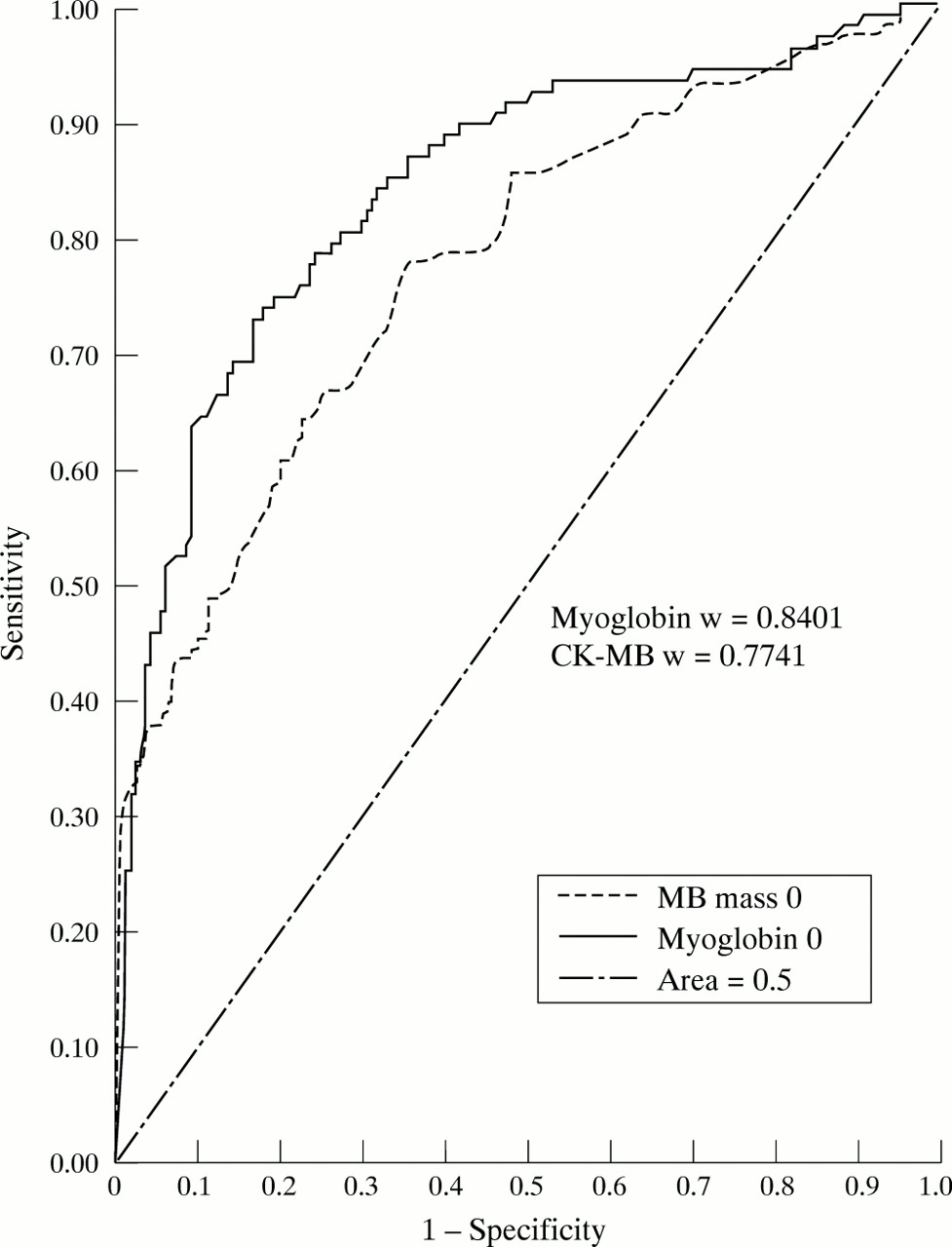
The evaluation is not confined to disease vnon-disease but can be produced for any feature that can be divided into a binary classification of the characteristic under investigation. This will include other characteristics such as survivalv non-survival or, as we have used, ejection fraction above or below 40%. Although numeric data is often used, ROC curves can be constructed using interval (grouped data).10If two or more tests are to be compared, there are statistical techniques to compare the areas under the curve for significant differences (fig 2).11 The likelihood ratio corresponds to the tangent to the curve at any point.12

• Download figure
• Open in new tab
• Download powerpoint

Figure 2

Comparative ROC curves for CK-MB and myoglobin for diagnosis of AMI on admission.

ROC analysis is a robust and powerful methodology, which largely avoids the pitfalls of sensitivity and specificity described above. It cannot abolish the prevalence problem but serves to minimise it. It allows direct comparison of methods that use the same end point (whatever that may be providing it supports a binary categorisation of the test dataset). It should be used more widely.